I recently had the opportunity to implement the Ramer-Douglas-Peuker path simplification algorithm for a small project. The goal in path simplification is to return a path with significantly fewer points while still being a good approximation of the original input. It’s helpful in applications like tracking when your sample rate is high but not all of the subjects you’re tracking are moving very quickly.

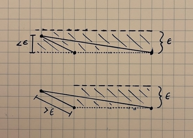
This algorithm works by first determining which point in the path is farthest from the line segment that connects the path’s endpoints. If the distance between this point and the segment is less than some pre-set threshold, we know that all other points in the path are also less than that threshold and we can remove them from the final, simplified path. If the distance of the farthest point is above the threshold, we mark that point for inclusion in the final path and run the same procedure on both sides of the point we’ve been considering. Below is a really fantastic visual representation of the algorithm from the wikipedia page courtesy of Mysid.¹

The algorithm, itself, is fairly simple to implement. What’s a bit more tricky is validating that it actually works. So, we’re going to use this path simplification algorithm as a practical way to explore strategies for building confidence that what we’ve written really behaves in the way we expect it to. We’re not going to discuss formal verification or techniques that are fully rigorous. Instead, we’re going to consider strategies that give fast feedback during early development, and these should be useful in a wider range of geometric algorithms than just path simplification.

Building Confidence

Let’s say we have written such an algorithm with the following signature.

def simplify_path(points: np.ndarray, epsilon: float) -> list[int]:
    # ...

That is, given an array of 3D points and some \epsilon > 0 that defines what it means for a point to be “too close” to the rest of the path to be included, our output will be a list of indexes in the original points array which constitute the final, simplified path.

We can first validate our algorithm with a few simple cases that are easy to hand-verify. Then, we’ll move on to some things that are more true-to-life in the length of the path or the structure they exhibit.

Simple cases

Sometimes unit tests have a bad reputation for being slow to write and brittle. That’s probably fair before the interface of a function has stabilized, but once it has, I find they actually speed up the process of feeling out whether our code is correct, especially when we don’t already have existing data to run against. The trick is finding the right tests to write.

It’s best to start small and validate our core primitives. Calculating the distance between a point and a line is an essential part of this algorithm, and we can test that extensively. Then, once we’ve removed a potential source of mistakes, we can move on to testing the path simplification function, itself. The goal here is to validate small cases that each constitute a fundamental, self-contained feature of our algorithm. Some examples include the following:²

• A point is far enough away from the line we’re testing against, so it should be included in the final path.
• A point is too close to the line, so it should be omitted in the final path.
• The farthest point from the line is too close, so it and all of its neighbors should be omitted in the final path.

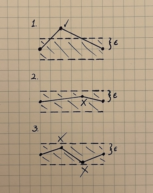
The first two examples can be represented with just three points. The third needs at least four, but these sorts of cases give us a quick sense of the baseline correctness of our function. The test code might look something like this.

def test_3_points_no_removal(self):
    path = np.array([[0, 0, 0], [5, 5, 5], [0, 0, 1]], dtype=np.float64)

    indexes = path_tools.simplify_path(path, epsilon=0.5)

    assert indexes == [0, 1, 2]


def test_3_points_middle_removed(self):
    path = np.array([[0, 0, 0], [1, 1, 1], [2, 2, 2]], dtype=np.float64)

    indexes = path_tools.simplify_path(path, epsilon=0.5)

    assert indexes == [0, 2]


def test_5_points_3_middle_removed(self):
    path = np.array(
        [[0, 0, 0], [1, 1, 1], [2, 2, 2], [3, 3, 3], [4, 4, 4]], dtype=np.float64
    )

    indexes = path_tools.simplify_path(path, epsilon=0.5)

    assert indexes == [0, 4]

Not every geometry problem lends itself well to unit testing, but in my experience, there’s almost always a simple case we can evaluate. Not every test has to be exact, either. We can write conditionals that validate characteristics of the output we know ought to be true without necessarily specifying what the precise output should be (e.g. all output points should be in this half-space). Whether we’re testing attributes of the output or validating the precise output, itself, our tests can function as more of a conversation with the code rather than a burdensome chore, and once they’re written, they continue to provide fast feedback as we rework any issues we find.

Visualizations

Unfortunately, we usually run out of small, simple test cases very quickly. When this happens, we can turn to real-world data or to something that we generate ourselves. In either case, there’s always a difficult question to address: how do we verify correctness when running against inputs with no ground-truth solution? There’s no easy answer to this question, but there is a shortcut—visualization.

This may seem incredibly unsatisfying because we would, of course, like perfect accuracy rather than ad-hoc verification, but building a good visualization is often a very efficient use of time. It makes a large amount of information easy to consume, which in turn allows us to be guided by data-supported intuition. This is a great place to be in the early stages of a newly created algorithm.³

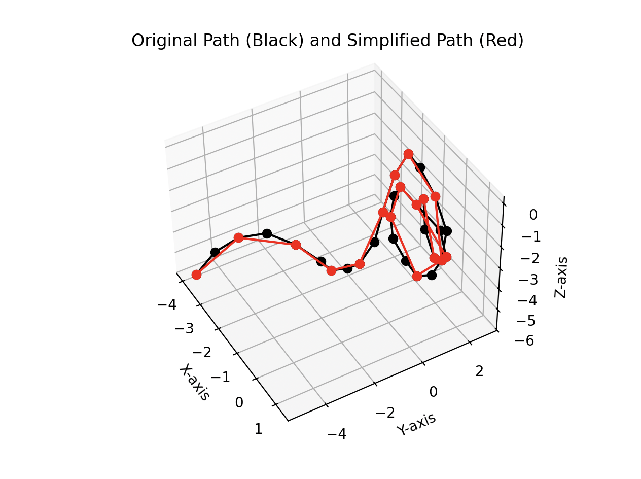
Thankfully in our case, this is an easy problem to visualize. We can draw both the input path and the simplified path overlayed together to help us see which points have been removed.

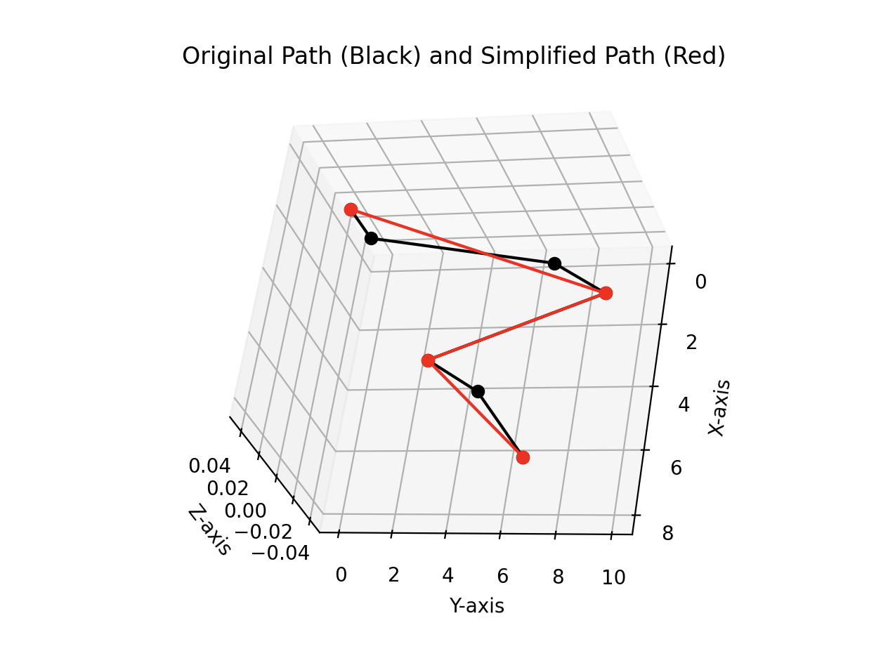
Now when we move on to generating test data, we’ll have a quick way to check the output against the original path.⁴

Generating Random Paths

Simple, hand-created test cases are effective for evaluating what we know we want to test, but they’re entirely useless for evaluating what we don’t realize we need to test. Carefully applied randomness can give us a wider range of inputs that helps to uncover unexpected issues. We can either create fully random inputs or inputs that, while random, are still constrained to look more like real-world data. Both can be useful.

Fully Random Paths

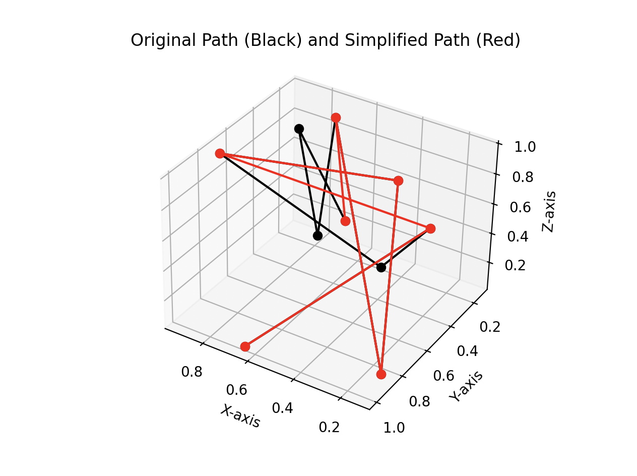
For path simplification, it’s especially easy to generate random paths, because any array of points is a valid (albeit chaotic) path.

def generate_random_path(
    n: int, scale: float = 1.0, seed: int | None = None
) -> np.ndarray:
    """
    Generates totally random 3D points.

    This is the easiest way to generate a path, but it isn't very
    representative of real-world data.
    """
    rng = np.random.default_rng(seed)
    return scale * rng.random((n, 3))

Note that it’s especially important to seed the random-number generator or at least print the seed that it derives. If we generate an interesting input that uncovers an issue but can’t replicate it, we won’t be able to verify the fix as easily.

Despite the fact that this looks entirely contrived, less true-to-life data sometimes helps to break our preconceptions. When testing with random paths, I found that I had unknowingly been using point-line distance instead of point-segment distance. This distinction is important when a point is close to the line that connects its neighbors but far from the segment that connects them.

Using point-line distance, this point would be removed, and this is likely the opposite of what we want from an algorithm that’s supposed to preserve interesting features. It’s often hard to find these cases without testing against data that’s very different than what a path is “supposed” to look like.

Constrained Random Paths

We can also create paths that obey certain constraints to make what we generate look more like real-world data. Let’s say we’re hoping to emulate the paths of people moving through grocery stores. Usually, people don’t make sharp changes in direction. They also don’t start and stop abruptly. Changes in velocity happen gradually, and there’s a low ceiling on the speed at which we expect people to move. We still want the paths to be randomized, but now, instead of picking any collection of points, we need to pick the next random point in a way that fits with these expectations.

We can do this by randomizing certain attributes of the next point. For instance, if we already have two points, we can calculate from those a direction and randomly perturb its angle. We can also randomize the distance traveled in the next step within a range of the previous distance. With those two abilities in hand, we can create paths that don’t look as wild as when they are fully randomly generated.

The code to generate these paths is a little bit more involved, especially when it comes to selecting the next angle in the path. There are lots of different ways to rotate points and vectors. In this case, it seemed easiest to use rotation matrices, but there are plenty of library calls that would accomplish the same thing.

def generate_constrained_random_path(
    n: int, max_angle: float = math.pi / 4, seed: int | None = None
) -> np.ndarray:
    """
    Build a path that looks a little bit more like the path a person
    would take by making the next point in the list move in roughly the
    same direction as the previous two points.
    """
    rng = np.random.default_rng(seed)

    if n == 0:
        return np.array([])
    if n == 1:
        return rng.random((1, 3))

    starting_point = rng.random(3)

    # Start with two random points one unit length away from each other.
    # Choose a random direction for the second point.
    tx, ty, tz = rng.random(3) * 2 * math.pi
    R = build_3d_rotation_matrix(tx, ty, tz)
    points = [starting_point, starting_point + (R @ np.array([1, 0, 0]))]

    for i in range(n - 2):
        tx, ty, tz = rng.random(3) * math.pi / 4
        R = build_3d_rotation_matrix(tx, ty, tz)

        prev_point = points[-1]
        prev_prev_point = points[-2]
        v = prev_point - prev_prev_point

        # So that the lengths of vectors have some variation,
        # scale v by a random factor.
        scaled_v = (rng.random(1) * 0.4 + 0.8) * v

        new_point = prev_point + R @ scaled_v
        points.append(new_point)

    return np.array(points)

These paths don’t look exactly like something in the real world, especially since we’re allowing for rotations around all three axes, but they’re definitely closer. And if we wanted to change the types of paths that we generate, we now have the beginnings of a framework for that.

Conclusion

Once we’ve gone through these or similar strategies to build confidence in the correctness of our implementation, we can determine whether greater rigor is necessary. Sometimes it is, but even in that case, it’s good to have reached the point of being functional as quickly as possible.

To view the code that supports this article, see this repository.

Appendix: Calculating Distances

While the article, itself, is focused on testing strategies, the way we calculate distance from a given point to a line is interesting enough to deserve it’s own section. As it turns out, there are lots of different ways to do this, but I like a particular vector formulation that we’ll work through below. Note, however, that it only works with 2D and 3D points.

Point-line distance

Calculating the point-line distance with vectors relies on our recollection of some basic area formulas and a fact or two about the cross product of two vectors.

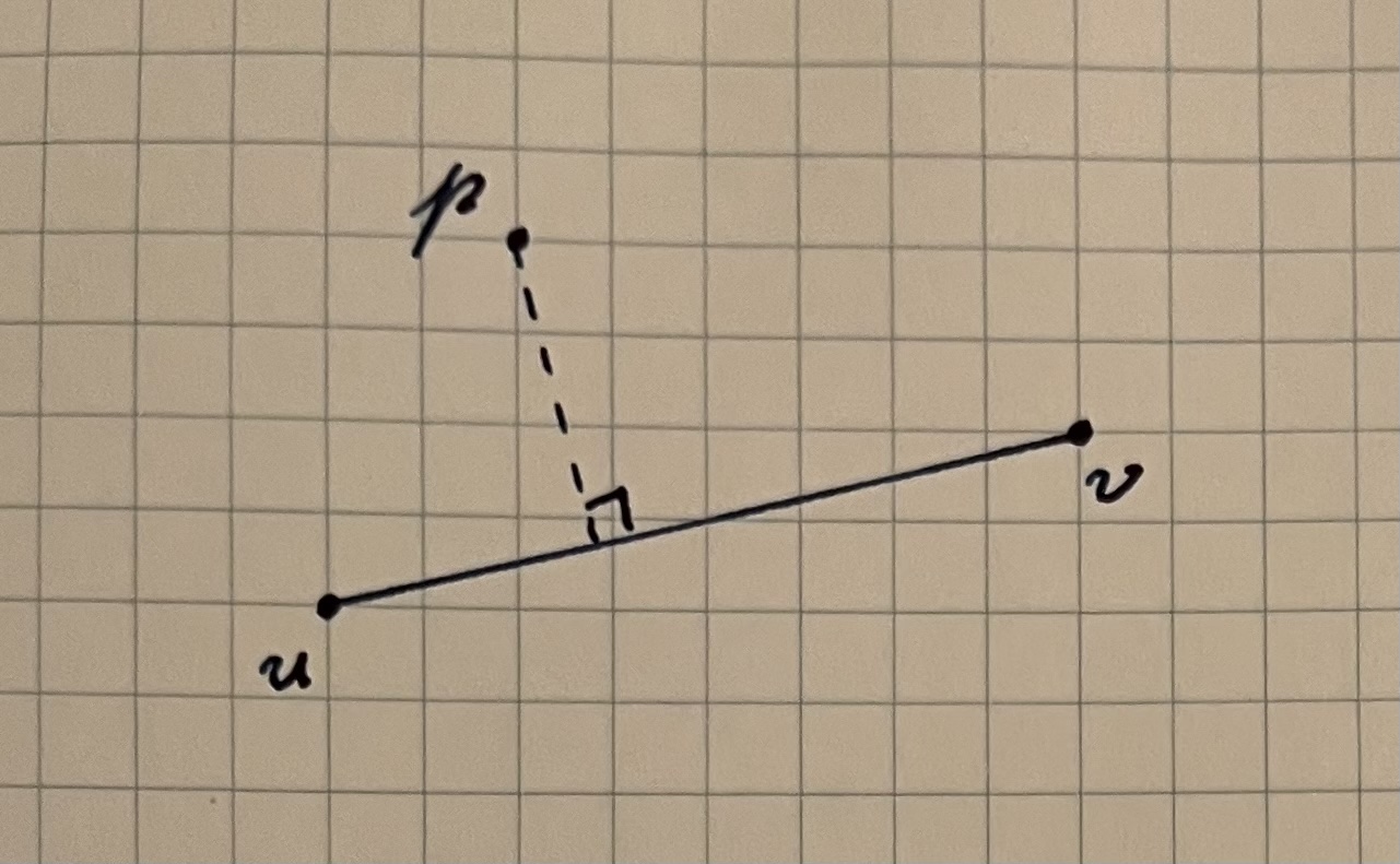
Let’s call the two points that define our line u and v, and let p be the point whose distance from the line we want to calculate. We’ll assume all of these points are in 3D for now, although we’ll show that this same method can work for 2D points as long as we write the code with a bit of care.

We can form two vectors from u to p and from u to v, which we’ll call \overrightarrow{up} and \overrightarrow{uv}. The magnitude of their cross product is equal to the area of the unique parallelogram that they define.

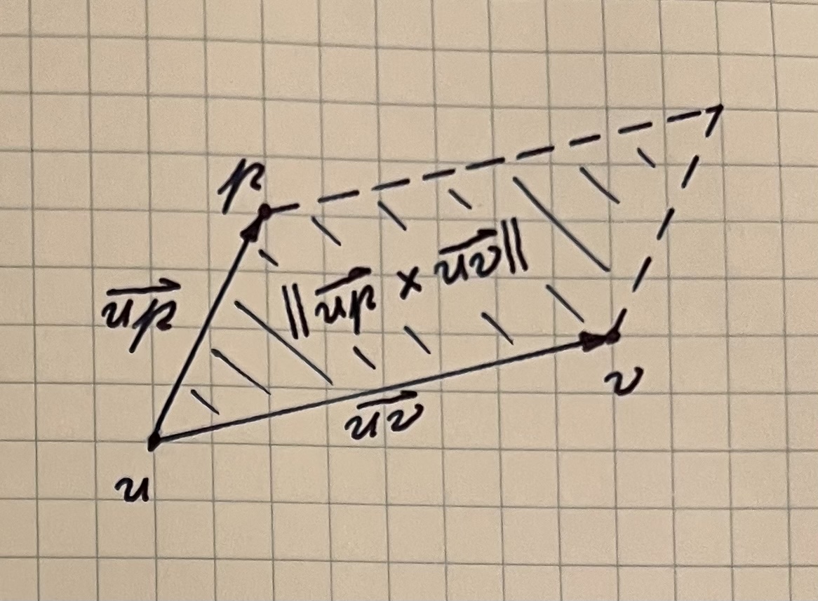
If we dig back in our mind for some dusty geometry formulas, we’ll recall that the area of a parallelogram can also be calculated by multiplying its base and its height.

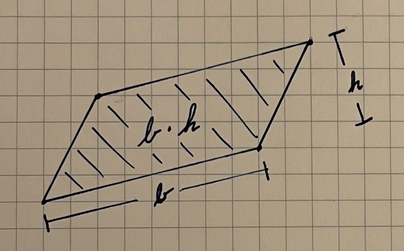
Going back to our original points, the length of \overrightarrow{uv} is the length of the base of our parallelogram. So, dividing the area from the cross product by the length of the base gives us the height. This height is equivalent to the distance from the line \overleftrightarrow{uv} to the point p.

The full formula is as follows:

\text{dist}(\overleftrightarrow{uv}, p) = \frac{\lVert \overrightarrow{up} \times \overrightarrow{uv} \rVert} {\lVert \overrightarrow{uv} \rVert}

Technically, the cross product is only defined in 3D, but we can get around this in 2D by forming 3D vectors with 0 as the z-component. Taking the cross product of two vectors (x, y, 0) and (u, v, 0) still gives us a vector whose magnitude is equal to the area we’re after.⁵

Point-segment distance

The formula we just described gives us point-line distance, but this may not be what we actually want. There are cases in which a point may be very close to the line connecting two points, but very far from the segment connecting them. In this case, we probably want to keep the point in our simplified path because it’s an interesting feature.

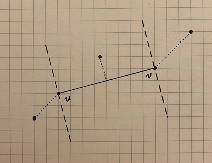
If the point p we’re evaluating is “between” the endpoints u and v of the segment, we can use point-line distance. If the point is on one side or the other, the shortest distance to the segment is the distance from p to u or p to v.

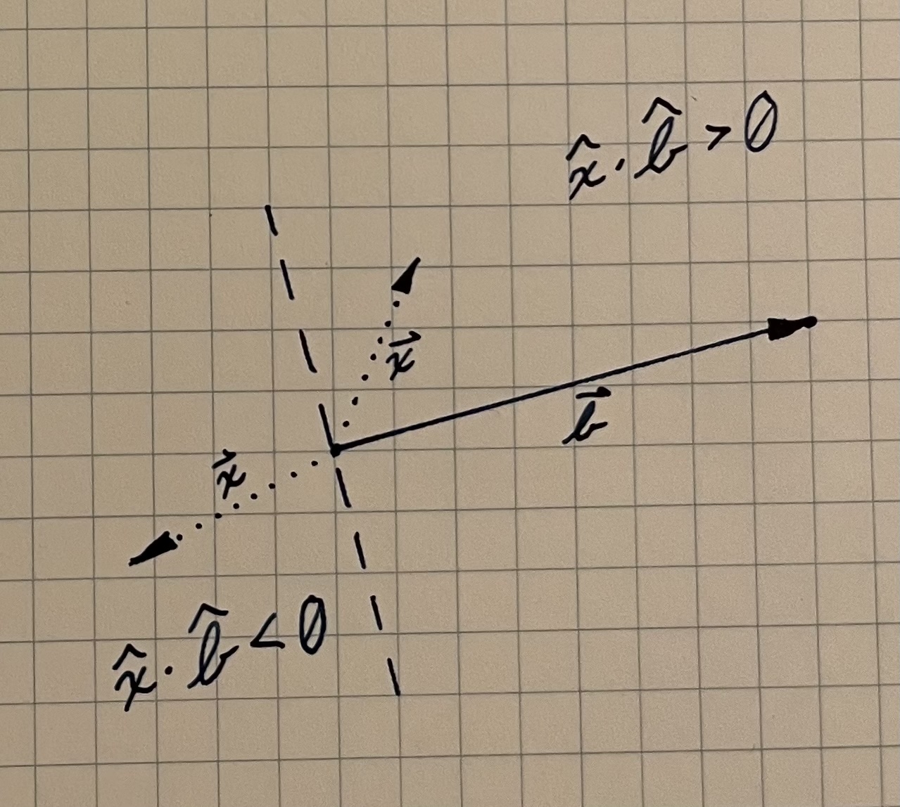
To know which case applies, we need a test to determine where p lies in relation to the other two points. The dot product between two vectors \overrightarrow{a} and \overrightarrow{b} is equal to \lVert \overrightarrow{a} \rVert \lVert \overrightarrow{b} \rVert \cos{\theta}, and that embedded \cos{\theta} can help us to find the relationship between these points.

In the diagram below, we see that whatever the magnitude of the two vectors may be, the \cos{\theta} component means that the dot product is positive when the angle between the two vectors is acute and negative when the angle between the vectors is obtuse. This gives us a way to see whether our point p lies to the “right” or “left” of one of the endpoints of our segment.

We can once again form two vectors \overrightarrow{up} and \overrightarrow{uv}. The dot product \overrightarrow{up} \cdot \overrightarrow{uv} will tell us about the relationship between u and p. Then, we need to do the same thing with the vectors \overrightarrow{vp} and \overrightarrow{vu} to determine the relationship between v and p. If p lies to the right of u and to the right of v, we can use \text{dist}(p,v) as our point-segment distance. If p lies to the left of both u and v, we can use \text{dist}(u,p). Otherwise, we can use point-line distance.